Code
# Load packages
library(tourr)
library(cassowaryr)
library(spinebil)
library(ferrn)
library(dplyr)
library(tidyr)
library(purrr)
library(ggplot2)skinny is suitable as a projection pursuit indexBefore using skinny inside a guided tour, I first check whether it behaves like a useful projection pursuit index.
For data matrix \(X \in \mathbb{R}^{n \times p}\) and projection basis \(A \in \mathbb{R}^{p \times 2}\), the projected data are
\[ Y = XA. \]
The projection pursuit index is then calculated on \(Y\).
Here I compare two versions of the index:
skinny(rescale = FALSE): the original skinny index.skinny(rescale = TRUE): a rescaled version designed to reduce the influence of values that commonly arise from Gaussian noise.In previous work, I estimated the distribution of the skinny index under bivariate Gaussian noise across different sample sizes. Using the estimated upper tail of this noise distribution, I derived a sample-size-dependent threshold
\[ \ell(n)=0.72-0.19\log(n)+0.02\{\log(n)\}^2, \]
The rescaled index is then defined as
\[ I_{\text{rescaled}} = \max \left( 0, \frac{I - \ell(n)} {1 - \ell(n)} \right), \]
where \(I\) is the original stringy05 value.
This transformation preserves the upper end of the index while shrinking values that are likely to arise from Gaussian noise. Values below the estimated noise threshold are mapped to zero, and values above the threshold are linearly rescaled to the interval \([0,1]\).
The motivation is that random noise projections can sometimes produce non-zero stringy values, potentially making optimisation more difficult. By incorporating an estimated noise threshold, the rescaled version aims to increase separation between structured projections and noise projections, allowing the optimiser to focus more strongly on projections containing genuine skinny structure.
# Load packages
library(tourr)
library(cassowaryr)
library(spinebil)
library(ferrn)
library(dplyr)
library(tidyr)
library(purrr)
library(ggplot2)rescale_skinny <- function(z, n) {
lb <- 0.72 - 0.19 * log(n) + 0.02 * (log(n)^2)
pmax(0, (z - lb) / (1 - lb))
}
skinny_index <- function(rescale = FALSE) {
function(mat) {
z <- cassowaryr::sc_skinny(mat[, 1], mat[, 2])
if (rescale) {
z <- rescale_skinny(z, nrow(mat))
}
z
}
}
skinny_index_raw <- skinny_index(rescale = FALSE)
skinny_index_rescaled <- skinny_index(rescale = TRUE)I use four datasets:
make_poly_data <- function(n = 300, p = 4, degree = 2, seed = 1050,
signal_noise_sd = 0.005) {
set.seed(seed)
t <- seq(-1, 1, length.out = n)
signal <- poly(t, degree = degree, raw = TRUE)
x <- matrix(rnorm(n * p), nrow = n, ncol = p)
x[, 2] <- signal[, 1] + rnorm(n, sd = signal_noise_sd)
x[, 3] <- signal[, 2] + rnorm(n, sd = signal_noise_sd)
colnames(x) <- paste0("V", seq_len(p))
as.data.frame(x)
}
dat4 <- scale(make_poly_data(n = 300, p = 4, degree = 2, seed = 1050))The polynomial signal is in variables 2 and 3.
basis_poly_true <- spinebil::basis_matrix(2, 3, 4)
basis_poly_noise <- spinebil::basis_matrix(1, 4, 4)For these spinebil datasets, I use six variables. The structured variables are V5 and V6, and the nuisance variables are V1, V2, V3, and V4.
set.seed(1050)
pipe_dat <- spinebil::pipe_data(300, 6) |> scale()
sine_dat <- spinebil::sin_data(300, 6, 1) |> scale()
spiral_dat <- spinebil::spiral_data(300, 6) |> scale()
basis_spinebil_true <- spinebil::basis_matrix(5, 6, 6)
basis_spinebil_noise1 <- spinebil::basis_matrix(1, 2, 6)
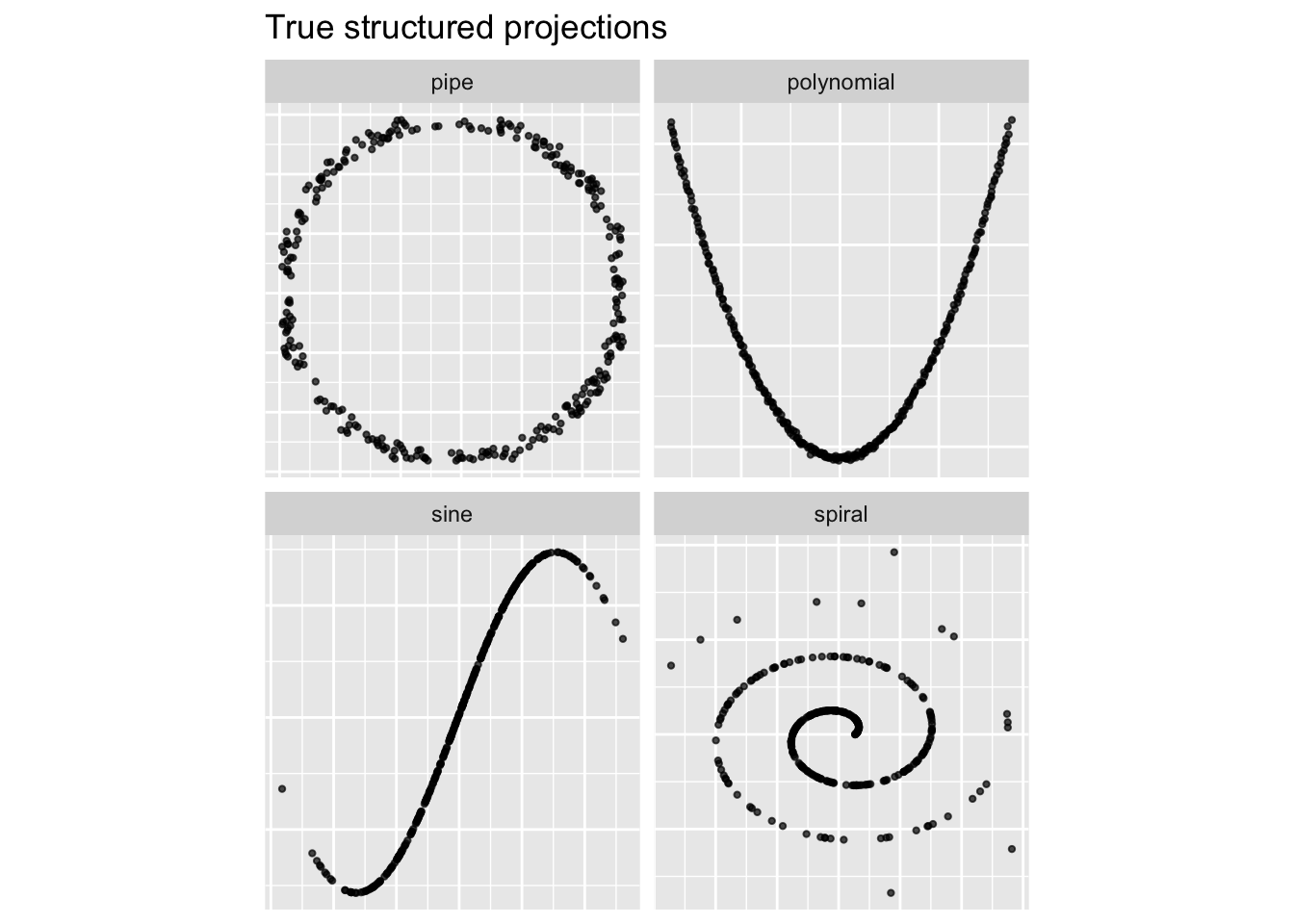
basis_spinebil_noise2 <- spinebil::basis_matrix(3, 4, 6)Before using the guided tour, I first plotted the signal variables directly. This is the target structures that I want the guided tour to find.
poly_plot <- as.data.frame(dat4) |>
transmute(x = V2, y = V3, data = "polynomial")
pipe_plot <- as.data.frame(pipe_dat) |>
transmute(x = V5, y = V6, data = "pipe")
sine_plot <- as.data.frame(sine_dat) |>
transmute(x = V5, y = V6, data = "sine")
spiral_plot <- as.data.frame(spiral_dat) |>
transmute(x = V5, y = V6, data = "spiral")
bind_rows(poly_plot, pipe_plot, sine_plot, spiral_plot) |>
ggplot(aes(x = x, y = y)) +
geom_point(size = 0.8, alpha = 0.7) +
facet_wrap(~ data, scales = "free") +
theme(
aspect.ratio = 1,
axis.text = element_blank(),
axis.ticks = element_blank()
) +
labs(
x = NULL,
y = NULL,
title = "True structured projections"
)
rescale_skinny <- function(z, n) {
  lb <- 0.72 - 0.19 * log(n) + 0.02 * (log(n)^2)
  pmax(0, (z - lb) / (1 - lb))
}

skinny_index <- function(rescale = FALSE) {
  function(mat) {

    z <- cassowaryr::sc_skinny(mat[, 1], mat[, 2])

    if (rescale) {
      z <- rescale_skinny(z, nrow(mat))
    }

    z
  }
}

skinny_index_raw <- skinny_index(rescale = FALSE)
skinny_index_rescaled <- skinny_index(rescale = TRUE)
direct_check <- tibble(
data = c("polynomial", "pipe", "sine", "spiral"),
raw_signal = c(
skinny_index_raw(dat4 %*% basis_poly_true),
skinny_index_raw(pipe_dat %*% basis_spinebil_true),
skinny_index_raw(sine_dat %*% basis_spinebil_true),
skinny_index_raw(spiral_dat %*% basis_spinebil_true)
),
raw_noise = c(
skinny_index_raw(dat4 %*% basis_poly_noise),
skinny_index_raw(pipe_dat %*% basis_spinebil_noise1),
skinny_index_raw(sine_dat %*% basis_spinebil_noise1),
skinny_index_raw(spiral_dat %*% basis_spinebil_noise1)
),
rescaled_signal = c(
skinny_index_rescaled(dat4 %*% basis_poly_true),
skinny_index_rescaled(pipe_dat %*% basis_spinebil_true),
skinny_index_rescaled(sine_dat %*% basis_spinebil_true),
skinny_index_rescaled(spiral_dat %*% basis_spinebil_true)
),
rescaled_noise = c(
skinny_index_rescaled(dat4 %*% basis_poly_noise),
skinny_index_rescaled(pipe_dat %*% basis_spinebil_noise1),
skinny_index_rescaled(sine_dat %*% basis_spinebil_noise1),
skinny_index_rescaled(spiral_dat %*% basis_spinebil_noise1)
)
)
knitr::kable(direct_check, digits = 3)| data | raw_signal | raw_noise | rescaled_signal | rescaled_noise |
|---|---|---|---|---|
| polynomial | 0.905 | 0.195 | 0.867 | 0.000 |
| pipe | 0.845 | 0.186 | 0.782 | 0.000 |
| sine | 0.819 | 0.271 | 0.745 | 0.000 |
| spiral | 0.503 | 0.306 | 0.303 | 0.027 |
plot_proj <- function(dat, basis, data, projection) {
  as.data.frame(as.matrix(dat) %*% basis) |>
    setNames(c("x", "y")) |>
    mutate(data = data, projection = projection)
}

projection_plot_data <- bind_rows(
  plot_proj(dat4, basis_poly_true, "polynomial", "signal"),
  plot_proj(dat4, basis_poly_noise, "polynomial", "noise"),
  plot_proj(pipe_dat, basis_spinebil_true, "pipe", "signal"),
  plot_proj(pipe_dat, basis_spinebil_noise1, "pipe", "noise"),
  plot_proj(sine_dat, basis_spinebil_true, "sine", "signal"),
  plot_proj(sine_dat, basis_spinebil_noise1, "sine", "noise"),
  plot_proj(spiral_dat, basis_spinebil_true, "spiral", "signal"),
  plot_proj(spiral_dat, basis_spinebil_noise1, "spiral", "noise")
)

ggplot(projection_plot_data, aes(x = x, y = y)) +
  geom_point(size = 0.8, alpha = 0.7) +
  facet_grid(projection ~ data, scales = "free")  +
  theme(
    aspect.ratio = 1,
    axis.text = element_blank(),
    axis.ticks = element_blank()
  ) +
  labs(
    x = NULL,
    y = NULL,
    title = "Signal and noise projections"
  )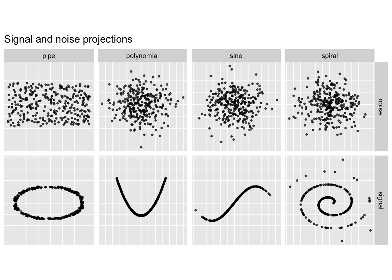
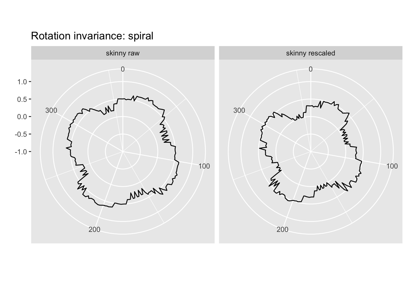
A useful projection pursuit index should give larger values to the signal projection than to the noise projection. The rescaled version should reduce the values assigned to noise projections.
For a 2D guided tour, the index should measure the plane, not the orientation inside the plane. This means rotating the projected 2D data should not substantially change the index value.
index_list <- list(
  skinny_index_raw,
  skinny_index_rescaled
)

index_labels <- c(
  "skinny raw",
  "skinny rescaled"
)

rotation_poly <- spinebil::profile_rotation(
  d = dat4 %*% basis_poly_true,
  index_list = index_list,
  index_labels = index_labels,
  n = 200
)

spinebil::plot_rotation(rotation_poly) +
  ggtitle("Rotation invariance: polynomial")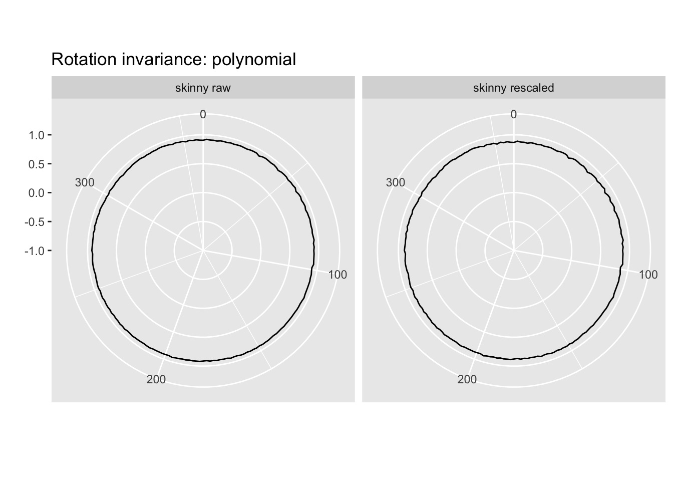
For the other datasets:
rotation_pipe <- spinebil::profile_rotation(
  d = pipe_dat %*% basis_spinebil_true,
  index_list = index_list,
  index_labels = index_labels,
  n = 200
)

rotation_sine <- spinebil::profile_rotation(
  d = sine_dat %*% basis_spinebil_true,
  index_list = index_list,
  index_labels = index_labels,
  n = 200
)

rotation_spiral <- spinebil::profile_rotation(
  d = spiral_dat %*% basis_spinebil_true,
  index_list = index_list,
  index_labels = index_labels,
  n = 200
)

spinebil::plot_rotation(rotation_pipe) +
  ggtitle("Rotation invariance: pipe")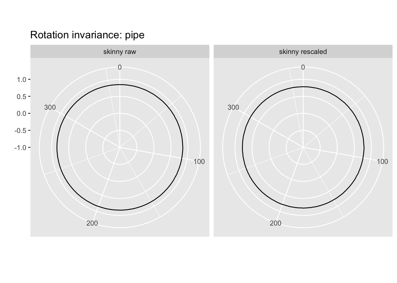
spinebil::plot_rotation(rotation_sine)  +
  ggtitle("Rotation invariance: sine")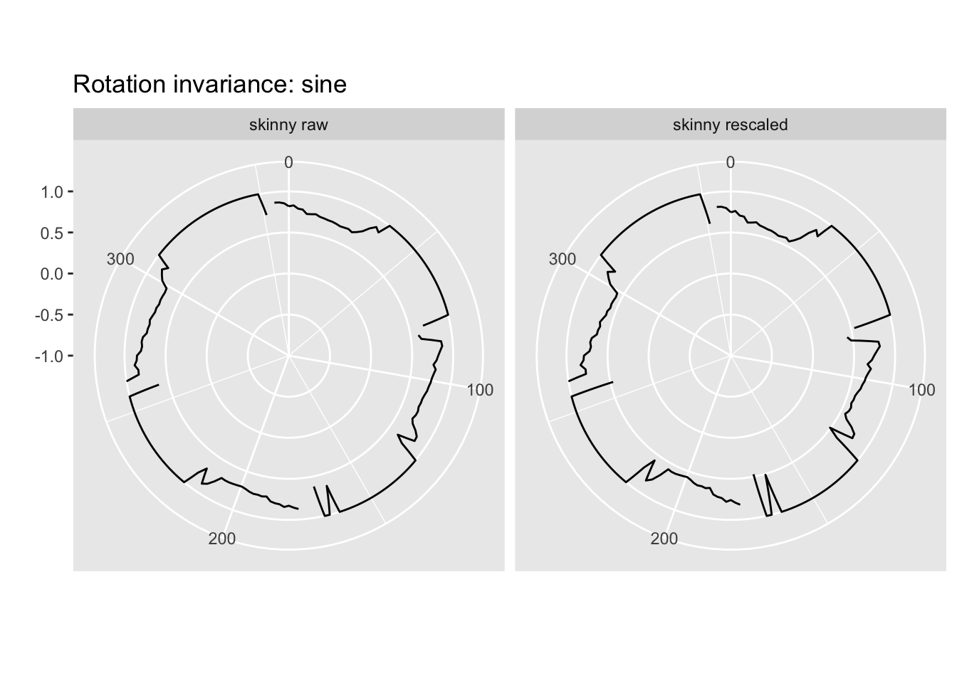
spinebil::plot_rotation(rotation_spiral) +
  ggtitle("Rotation invariance: spiral")