Testing Scagnostic Rescaling Across Preprocessing Settings

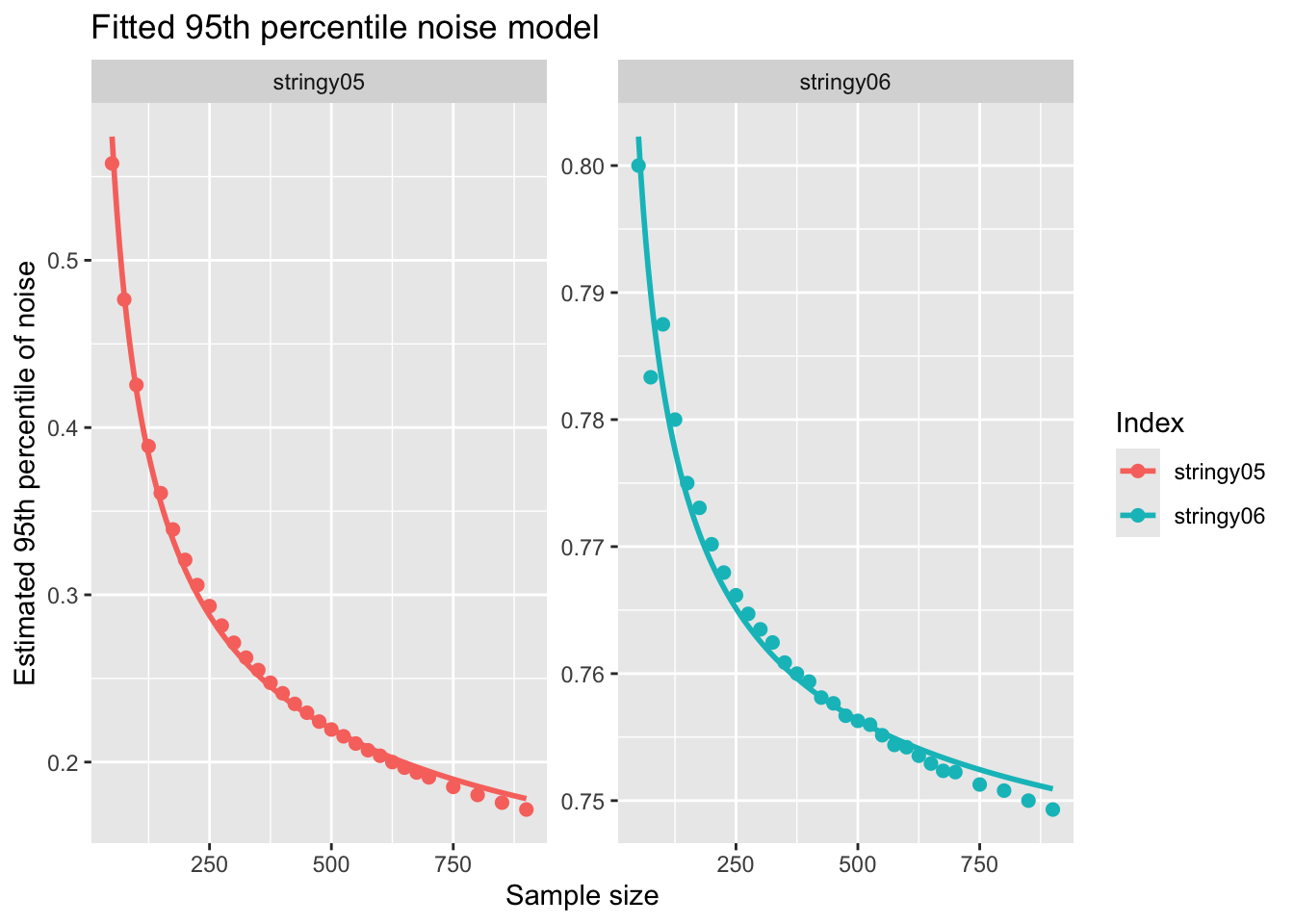
Exploring whether fitted 95th percentile noise models for scagnostic indices remain valid when cassowaryr preprocessing choices change.

Exploring Whether One Fitted Noise Model Is Enough Across Different Preprocessing Settings

In this blog post, I explore whether a single fitted model is sufficient for rescaling scagnostic indices under different preprocessing settings. I use the cassowaryr package to calculate scagnostics, which are useful for shape analysis and for identifying different types of structure in two-dimensional projections.

Previously, I ran my simulations using the CRAN version of cassowaryr, version 2.0.2. At that time, the preprocessing steps were different from the current GitHub version. In particular, the simulations were run without hexagonal binning, and outlier removal was implemented as a one-time preprocessing step. My estimated noise distributions, and therefore the fitted models I used for rescaling, were based on those preprocessing choices.

However, the current GitHub version of cassowaryr has changed. Hexagonal binning has been added, and outlier removal is now implemented iteratively rather than using the previous one-step approach. These changes matter because the 95th percentile of the noise distribution depends on the preprocessing applied before calculating the scagnostic indices.

The reason I estimate the 95th percentile of the noise distribution is to rescale the scagnostic indices. In theory, the lower bound of a scagnostic index should be zero. However, for bivariate Gaussian noise, where there is no meaningful visual pattern, the raw scagnostic values do not necessarily reach zero. Therefore, I use the estimated 95th percentile of the noise distribution as a reference point for rescaling. This allows the indices to be placed on a more comparable scale, especially when they are used in higher-dimensional projection pursuit.

In my previous work, I estimated these 95th percentile values for several sample sizes and fitted a model using the CRAN version of cassowaryr. Later, when I wanted to implement my own changes to the package and submit a pull request, I noticed that the preprocessing steps in the GitHub version had changed. This raised an important question:

Can the fitted model from the previous preprocessing setup still be used under the new preprocessing settings?

To investigate this, I tested whether the old fitted model still controlled the upper tail of the noise distribution. In particular, I counted how often noise-generated scagnostic values exceeded the fitted 95th percentile threshold. If the model worked well across all preprocessing settings, then I would expect roughly 5% of the simulated noise values to exceed the threshold.

However, this was not what I observed. The exceedance rate was not consistently close to 5% across the different combinations of hexagonal binning and outlier removal.

Because of this, I decided to rerun the simulations using the current GitHub version of cassowaryr, starting with the setting hex = FALSE and out_rm = FALSE. This is important because, in the previous CRAN version, “no outlier removal” was not the default behaviour in the same way, and the outlier removal method itself was different.

My goal is to write a general simulation workflow that is not hard-coded for only one index or one specific set of parameters. I want the same code structure to be reusable for other scagnostic indices, sample sizes, preprocessing options, and simulation settings. This will make it easier to compare noise distributions across different versions of the package and across different preprocessing choices.

In the next section, I describe the general simulation code I used to generate the noise distributions and estimate the 95th percentile values.

General simulation function for estimating the 95th percentile of noise

To make the simulation process reusable, I wrote a general function called estimate_95th(). The purpose of this function is to estimate the 95th percentile of the noise distribution for one or more scagnostic indices.

The function is general in several ways. First, it can take a list of different scagnostic functions. Second, it can run the same index under different preprocessing settings, such as hexagonal binning and outlier removal. Third, it can be used over a sequence of sample sizes. Finally, it can save intermediate results to a CSV file, which is useful because these simulations can take a long time to run.

In each simulation, I generate bivariate Gaussian noise. Since this type of data does not contain a meaningful visual pattern, it provides a useful baseline for understanding how large a scagnostic value can be under noise alone. For each sample size, preprocessing setting, and index, I repeat the simulation many times and estimate the empirical 95th percentile of the resulting noise values.

# General simulation function for estimating 95th percentile of noise 

estimate_95th <- function(
    index_funs,
    n_sim,
    n_start,
    n_end,
    step = 25,
    settings = list(default = list()),
    seed = 1028,
    workers = 1,
    output_file = NULL,
    index_args = list(),
    ...
) {
  
  extra_args <- list(...)
  
  if (is.function(index_funs)) {
    stop("Please provide index_funs as a named list, e.g. list(stringy05 = cassowaryr::sc_stringy05)")
  }
  
  if (is.null(names(index_funs)) || any(names(index_funs) == "")) {
    stop("index_funs must be a named list.")
  }
  
  if (is.null(names(settings)) || any(names(settings) == "")) {
    stop("settings must be a named list.")
  }
  
  sample_sizes <- seq(n_start, n_end, by = step)
  
  if (workers > 1) {
    with(future::plan(future::multisession, workers = workers), local = TRUE)
  } else {
    with(future::plan(future::sequential), local = TRUE)
  }
  
  if (!is.null(output_file)) {
    readr::write_csv(
      tibble(
        sample_size = numeric(),
        setting = character(),
        index = character(),
        p95 = numeric(),
        n_valid = numeric(),
        n_sim = numeric()
      ),
      output_file
    )
  }
  
  final_results <- list()
  
  for (n_obs in sample_sizes) {
    
    cat("Running sample size:", n_obs, "\n")
    
    raw_results <- furrr::future_map_dfr(
      seq_len(n_sim),
      function(i) {
        
        seed_i <- seed + i 
        set.seed(seed_i)
        
        mat <- cbind(
          rnorm(n_obs),
          rnorm(n_obs)
        )
        
        map_dfr(names(settings), function(setting_name) {
          
          setting_args <- settings[[setting_name]]
          
          map_dfr(names(index_funs), function(index_name) {
            
            index_fun <- index_funs[[index_name]]
            
            all_args <- c(
              setting_args,
              extra_args,
              index_args[[index_name]]
            )
            
            value <- tryCatch(
              {
                as.numeric(
                  do.call(
                    index_fun,
                    c(list(mat[, 1], mat[, 2]), all_args)
                  )
                )[1]
              },
              error = function(e) NA
            )
            
            tibble(
              sample_size = n_obs,
              simulation = i,
              seed = seed_i,
              setting = setting_name,
              index = index_name,
              value = value
            )
          })
        })
      },
      .options = furrr::furrr_options(seed = TRUE),
      .progress = TRUE
    )
    
    p95_results <- raw_results |>
      group_by(sample_size, setting, index) |>
      summarise(
        p95 = as.numeric(quantile(value, 0.95, na.rm = TRUE)),
        n_valid = sum(!is.na(value)),
        n_sim = n_sim,
        .groups = "drop"
      )
    
    if (!is.null(output_file)) {
      readr::write_csv(p95_results, output_file, append = TRUE)
    }
    
    final_results[[as.character(n_obs)]] <- p95_results
    
    cat("Finished sample size:", n_obs, "\n")
  }
  
  bind_rows(final_results)
}

For the simulations in this analysis, I used a base seed of 1028. I ran 100000 simulations for sample sizes from 50 to 900. Because the simulations were computationally expensive, I saved the results in several smaller CSV files, each covering a different range of sample sizes.

Combining the simulation results

After running the simulations, I combined all of the CSV files into one dataset.

files <- list.files(
  path = ".",
  pattern = "^samplesize_stringy_.*\\.csv$",
  full.names = TRUE
)


results_samplesize <- files |>
  map_dfr(\(f) {
    readr::read_csv(f, show_col_types = FALSE)
  }) |>
  arrange(sample_size, index)

Fitting a model to the estimated 95th percentiles

Once all the simulation results were combined, I fitted a model to describe how the estimated 95th percentile changes with sample size.

The fitted model uses the inverse square root of the sample size:

\[ p_{95}(n) = a + \frac{b}{\sqrt{n}}. \]

This model is useful because the noise threshold usually decreases as the sample size increases. By fitting a smooth model, I can estimate the 95th percentile for different sample sizes without needing to rerun the full simulation every time.

If I want to fit the model only for a particular preprocessing setting, for example no hexagonal binning and no outlier removal, I can filter the results before fitting:

df_fit <- results_samplesize |>
  filter(
    hex == "no",
    out_rm == "no"
  ) |>
  group_by(index, sample_size)|>
  mutate(
    inv_sqrt_n = 1 / sqrt(sample_size)
  )

Then I fit the linear model separately for each scagnostic index:

fit_results <- df_fit |>
  group_by(index) |>
  group_map(\(d, key) {
    fit <- lm(p95 ~ inv_sqrt_n, data = d)
    
    tibble(
      index = as.character(key$index),
      model = "a + b / sqrt(n)",
      a = unname(coef(fit)[1]),
      b = unname(coef(fit)[2]),
      r_squared = summary(fit)$r.squared
    )
  }) |>
  bind_rows()

fit_results

# A tibble: 2 × 5
  index     model                a     b r_squared
  <chr>     <chr>            <dbl> <dbl>     <dbl>
1 stringy05 a + b / sqrt(n) 0.0561 3.66      0.997
2 stringy06 a + b / sqrt(n) 0.735  0.475     0.977

The fitted coefficients can then be used to predict the 95th percentile noise threshold at any sample size:

pred_data <- expand_grid(
  index = unique(df_fit$index),
  sample_size = seq(
    min(df_fit$sample_size),
    max(df_fit$sample_size),
    by = 5
  )
) |>
  mutate(
    inv_sqrt_n = 1 / sqrt(sample_size)
  )

pred_results <- pred_data |>
  left_join(fit_results, by = "index") |>
  mutate(
    fitted_p95 = a + b * inv_sqrt_n
  )

Finally, I plotted the observed simulation-based 95th percentiles together with the fitted model.

ggplot(df_fit, aes(x = sample_size, y = p95, colour = index)) +
  geom_point(size = 2) +
  geom_line(
    data = pred_results,
    aes(y = fitted_p95),
    linewidth = 1
  ) +
facet_wrap(~ index, scales = "free") +
  labs(
    title = "Fitted 95th percentile noise model",
    x = "Sample size",
    y = "Estimated 95th percentile of noise",
    colour = "Index"
  )

This fitted model gives approximation to the simulated 95th percentile values. I can then compare whether the same fitted model is valid across different preprocessing settings, such as with or without hexagonal binning and with or without outlier removal.

stringy_500 <- read_csv("stringy_scale_500_10000.csv")

stringy_500_rescaled <- stringy_500 |>
  left_join(fit_results, by = "index") |>
  mutate(
    sample_size = n_final,
    lb = a + b / sqrt(sample_size),
    rescaled_value = (value - lb) / (1 - lb),
    rescaled_value = pmax(rescaled_value, 0)
  ) |> select(simulation:index , rescaled_value)

noise_positive_check <- stringy_500_rescaled |> 
  filter(sigma == "noise") |>
  group_by(index, hex, out_rm) |>
  summarise(
    n_noise = n(),
    n_positive = sum(rescaled_value> 0, na.rm = TRUE),
    false_positive_rate = n_positive / n_noise,
    expected_5_percent_count = 0.05 * n_noise,
    above_5_percent = false_positive_rate > 0.05,
    .groups = "drop"
  )

knitr::kable(noise_positive_check)

index	hex	out_rm	n_noise	n_positive	false_positive_rate	expected_5_percent_count	above_5_percent
stringy05	no	no	10000	504	0.0504	500	TRUE
stringy05	no	yes	10000	1071	0.1071	500	TRUE
stringy05	yes	no	10000	166	0.0166	500	FALSE
stringy05	yes	yes	10000	526	0.0526	500	TRUE
stringy06	no	no	10000	480	0.0480	500	FALSE
stringy06	no	yes	10000	767	0.0767	500	TRUE
stringy06	yes	no	10000	112	0.0112	500	FALSE
stringy06	yes	yes	10000	212	0.0212	500	FALSE

After fitting the inverse-square-root model to the estimated 95th percentiles, I checked whether the fitted threshold actually behaved like a 95th percentile. If the model were appropriate, approximately 5% of Gaussian noise simulations should exceed the fitted threshold. However, I observed exceedance rates larger than 5% in some cases. This suggests that the fitted model may be underestimating the empirical 95th percentile for some sample sizes or preprocessing settings. Therefore, the issue is not only the change in preprocessing; it may also be partly due to the fitted model not being flexible enough to capture the shape of the noise distribution across sample sizes.

Because of this, I decided to compare the original inverse-square-root model with several alternative models. The goal is to check whether a slightly more flexible model can better capture the shape of the simulated 95th percentile curve.

My original model was:

\[ p_{95}(n) = a + \frac{b}{\sqrt{n}}. \]

This is simple and interpretable, but it may be too restrictive if the empirical 95th percentile curve bends more strongly for small or medium sample sizes. Therefore, I compare it with a few alternatives:

\[ p_{95}(n) = a + \frac{b}{\sqrt{n}} + \frac{c}{n}, \]

a log-quadratic model,

\[ p_{95}(n) = a + b \log(n) + c \log(n)^2, \]

and natural spline models, which are more flexible.

library(tidyverse)
library(broom)
library(splines)

df_model <- results_samplesize |>
  mutate(
    inv_sqrt_n = 1 / sqrt(sample_size),
    inv_n = 1 / sample_size,
    logn = log(sample_size),
    logn2 = log(sample_size)^2
  )

If I want to focus on one preprocessing setting first, for example no hexagonal binning and no outlier removal, I can filter the data before fitting the models:

df_model_no_hex_noout <- df_model |>
  filter(hex == "no", out_rm == "no")

Candidate models

fit_candidate_models <- function(d) {
  list(
    original_inv_sqrt = lm(
      p95 ~ inv_sqrt_n,
      data = d
    ),
    
    inv_sqrt_plus_inv_n = lm(
      p95 ~ inv_sqrt_n + inv_n,
      data = d
    ),
    
    log_quadratic = lm(
      p95 ~ logn + logn2,
      data = d
    ),
    
    spline_df3 = lm(
      p95 ~ splines::ns(sample_size, df = 3),
      data = d
    ),
    
    spline_df4 = lm(
      p95 ~ splines::ns(sample_size, df = 4),
      data = d
    )
  )
}

I then fit each candidate model separately for each scagnostic index.

model_fits <- df_model_no_hex_noout |>
  group_by(index) |>
  nest() |>
  mutate(
    fits = map(data, fit_candidate_models)
  )

Compare model fit

To compare the models, I calculate standard model summaries such as \(R^2\), adjusted \(R^2\), AIC, BIC, and residual standard error. I also compute RMSE directly from the fitted residuals.

model_comparison <- model_fits |>
  mutate(
    metrics = map(fits, \(fit_list) {
      imap_dfr(fit_list, \(fit, model_name) {
        glance(fit) |>
          mutate(
            model = model_name,
            r_squared = r.squared,
            adj_r_squared = adj.r.squared,
            AIC = AIC,
            BIC = BIC,
            sigma = sigma,
            RMSE = sqrt(mean(residuals(fit)^2))
          )
      })
    })
  ) |>
  select(index, metrics) |>
  unnest(metrics) |>
  arrange(index, AIC)

A better model should have lower AIC, lower BIC, lower RMSE, and residuals that do not show a strong systematic pattern.

overall_best_models <- model_comparison |>
  group_by(index) |>
  mutate(
    rank_AIC = min_rank(AIC),
    rank_BIC = min_rank(BIC),
    rank_RMSE = min_rank(RMSE),
    total_rank = rank_AIC + rank_BIC + rank_RMSE
  ) |>
  slice_min(total_rank, n = 1, with_ties = FALSE) |>
  ungroup() |> 
  select(index, model)

overall_best_models

# A tibble: 2 × 2
  index     model              
  <chr>     <chr>              
1 stringy05 inv_sqrt_plus_inv_n
2 stringy06 log_quadratic      

best_model_spec <- tribble(
  ~index,      ~model,
  "stringy05", "inv_sqrt_plus_inv_n",
  "stringy06", "log_quadratic"
)

fit_selected_model <- function(data, model_name) {
  if (model_name == "inv_sqrt_plus_inv_n") {
    lm(p95 ~ inv_sqrt_n + inv_n, data = data)
  } else if (model_name == "log_quadratic") {
    lm(p95 ~ logn + logn2, data = data)
  }
}

best_fits <- best_model_spec |>
  mutate(
    data = map(index, \(idx) {
      df_model_no_hex_noout |>
        filter(index == idx)
    }),
    fit = map2(data, model, fit_selected_model)
  )


best_coefficients <- best_fits |>
  mutate(
    coefficients = map(fit, broom::tidy)
  ) |>
  select(index, model, coefficients) |>
  unnest(coefficients)

best_coefficients

# A tibble: 6 × 7
  index     model               term       estimate std.error statistic  p.value
  <chr>     <chr>               <chr>         <dbl>     <dbl>     <dbl>    <dbl>
1 stringy05 inv_sqrt_plus_inv_n (Intercep…  0.0259   0.000523     49.5  8.42e-29
2 stringy05 inv_sqrt_plus_inv_n inv_sqrt_n  4.59     0.0153      301.   1.11e-50
3 stringy05 inv_sqrt_plus_inv_n inv_n      -5.89     0.0949      -62.1  1.55e-31
4 stringy06 log_quadratic       (Intercep…  0.924    0.0131       70.6  4.35e-33
5 stringy06 log_quadratic       logn       -0.0409   0.00480      -8.52 2.89e- 9
6 stringy06 log_quadratic       logn2       0.00223  0.000434      5.15 1.85e- 5

best_coef_wide <- best_coefficients |>
  mutate(
    term = case_when(
      term == "(Intercept)" ~ "intercept",
      TRUE ~ term
    )
  ) |>
  select(index, model, term, estimate) |>
  pivot_wider(
    names_from = term,
    values_from = estimate,
    names_prefix = "beta_"
  )

best_coef_wide

# A tibble: 2 × 7
  index     model beta_intercept beta_inv_sqrt_n beta_inv_n beta_logn beta_logn2
  <chr>     <chr>          <dbl>           <dbl>      <dbl>     <dbl>      <dbl>
1 stringy05 inv_…         0.0259            4.59      -5.89   NA        NA      
2 stringy06 log_…         0.924            NA         NA      -0.0409    0.00223

stringy_500 <- readr::read_csv("stringy_scale_500_10000.csv")

stringy_500_rescaled <- stringy_500 |>
  left_join(best_coef_wide, by = "index") |>
  mutate(
    sample_size = n_final,
    inv_sqrt_n = 1 / sqrt(sample_size),
    inv_n = 1 / sample_size,
    logn = log(sample_size),
    logn2 = log(sample_size)^2,
    
    lb = case_when(
      model == "inv_sqrt_plus_inv_n" ~ 
        beta_intercept + beta_inv_sqrt_n * inv_sqrt_n + beta_inv_n * inv_n,
      
      model == "log_quadratic" ~ 
        beta_intercept + beta_logn * logn + beta_logn2 * logn2,
      
      TRUE ~ NA_real_
    ),
    
    rescaled_value = (value - lb) / (1 - lb),
    rescaled_value = pmax(rescaled_value, 0)
  ) |>
  select(simulation:index, lb, rescaled_value)

stringy_500_rescaled

# A tibble: 160,000 × 10
   simulation  seed sigma  hex   out_rm n_final value index    lb rescaled_value
        <dbl> <dbl> <chr>  <chr> <chr>    <dbl> <dbl> <chr> <dbl>          <dbl>
 1          2  1029 noise  no    no         500 0.169 stri… 0.219          0    
 2          2  1029 noise  no    no         500 0.731 stri… 0.756          0    
 3          2  1029 struc… no    no         500 1.000 stri… 0.219          1.000
 4          2  1029 struc… no    no         500 1     stri… 0.756          1    
 5          2  1029 noise  no    yes        486 0.179 stri… 0.222          0    
 6          2  1029 noise  no    yes        486 0.728 stri… 0.757          0    
 7          2  1029 struc… no    yes        499 1.000 stri… 0.220          1.000
 8          2  1029 struc… no    yes        499 1     stri… 0.756          1    
 9          2  1029 noise  yes   no         398 0.197 stri… 0.241          0    
10          2  1029 noise  yes   no         398 0.716 stri… 0.759          0    
# ℹ 159,990 more rows

exceedance_count <- stringy_500 |>
  left_join(best_coef_wide, by = "index") |>
  mutate(
    inv_sqrt_n = 1 / sqrt(n_final),
    inv_n = 1 / n_final,
    logn = log(n_final),
    logn2 = log(n_final)^2,
    
    lb = case_when(
      model == "inv_sqrt_plus_inv_n" ~ 
        beta_intercept + beta_inv_sqrt_n * inv_sqrt_n + beta_inv_n * inv_n,
      
      model == "log_quadratic" ~ 
        beta_intercept + beta_logn * logn + beta_logn2 * logn2,
      
      TRUE ~ NA_real_
    ),
    
    exceeds_lb = value > lb
  ) |>
  group_by(index) |>
  summarise(
    n = sum(!is.na(value)),
    n_exceed = sum(exceeds_lb, na.rm = TRUE),
    exceedance_rate = n_exceed / n,
    exceeds_5_percent = exceedance_rate > 0.05,
    .groups = "drop"
  )

exceedance_count

# A tibble: 2 × 5
  index         n n_exceed exceedance_rate exceeds_5_percent
  <chr>     <int>    <int>           <dbl> <lgl>            
1 stringy05 79916    42078           0.527 TRUE             
2 stringy06 79917    41498           0.519 TRUE             

Copyright

Copyright © 2026 Tina Rashid Jafari. All rights reserved.